Practice

In order to utilise TiRex, make sure to either locally install it in your preferred Python environment or use a hosted Jupyter Notebook service like Google Colab.

1. Install Tirex

# install with the extra 'plotting' for plotting support
pip install 'tirex-ts[plotting]'

2. Import TiRex and supporting libraries

(Do this either in a Jupyter Notebook, a local Python file or directly in your Python Environment)

# standard imports
import pandas as pd
import numpy as np
import matplotlib.pyplot as plt

# TiRex specific imports
from tirex import load_model
from tirex.util import plot_forecast

# set default figure size for all plots
plt.rcParams['figure.figsize'] = (12, 6)

3. Load a TiRex model

Model weights are automatically fetched from HuggingFace

# load a TiRex model (automatically fetching the weights from HuggingFace)
model = load_model("NX-AI/TiRex")

4. Toy Example - Sine Wave

Use the plot_forecast utility function provided in our framework to visualise how the model behaves on a simple sine wave.

# generate a simple sine wave
sin = np.sin(np.arange(0, 10, 0.05))

# split sine wave into context (to be learnt from) and future values
prediction_length = 20
sin_context, sin_future = np.split(sin, [-prediction_length])

# make a forecast based on the context
# model.forecast() returns quantiles and a mean of the prediction
forecast_quantiles, forecast_mean = model.forecast(sin_context, prediction_length=prediction_length)

# shape of forecasts
forecast_quantiles.shape, forecast_mean.shape

(torch.Size([1, 20, 9]), torch.Size([1, 20]))

plot_forecast(
    context=sin_context,
    # we need to remove (squeeze) the batch dimension from the returned tensors
    forecasts=forecast_quantiles.squeeze(),
    ground_truth=sin_future
)

5. Forecasting with Sample Data and varying Prediction Length

With the code below, you can load some example data and generate forecasts. To understand the potential of TiRex it is important to experiment with the prediction_length parameter to see its effect.

Load Example Data

# load example data and split into context (to be learnt from) and future values
data_base_url = "https://raw.githubusercontent.com/NX-AI/tirex/refs/heads/main/tests/data/"

# short horizon example: air passengers per month
ctx_s, future_s = np.split(pd.read_csv(f"{data_base_url}/air_passengers.csv").values.reshape(-1), [-59])

Short Horizon Forecast

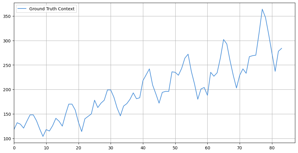
The short horizon forecast data example contains number of air passengers per month.

Visualize a short horizon data sample.

# plot time series
print("Short series (number of air passengers per month):")
plot_forecast(context=ctx_s)

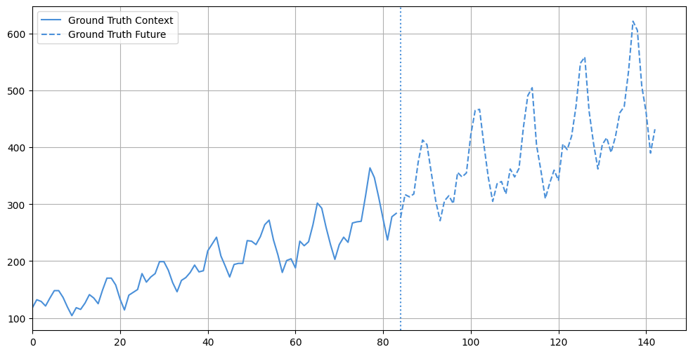
Visualize the short horizon data incuding future values

# plot time series with future values
print("Short series (number of air passengers per month):")
plot_forecast(context=ctx_s, ground_truth=future_s)

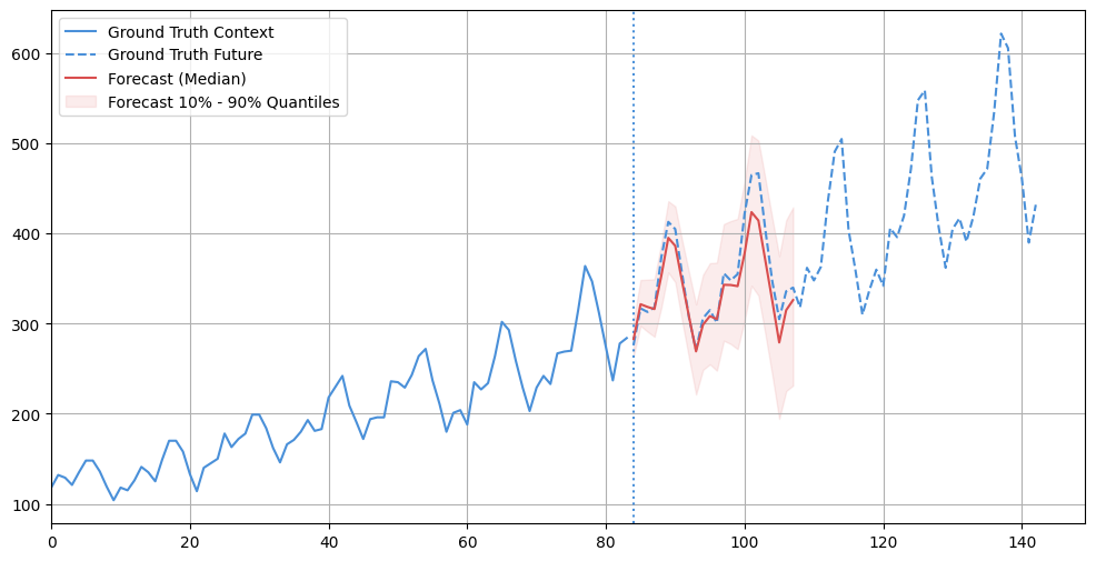
Make a forecast on the data, starting with a prediction length of 12

prediction_length = 12
quantiles_s, mean_s = model.forecast(ctx_s, prediction_length=prediction_length)

print(f"Short series (number of air passengers per month): {prediction_length=}")
plot_forecast(context=ctx_s, ground_truth=future_s, forecasts=quantiles_s[0])

Extend the prediction length

# extend prediction length to 24
prediction_length = 24

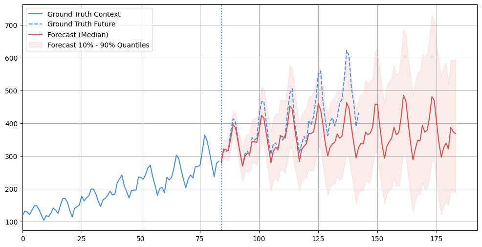
We can observe that very long prediction lengths can lead to higher uncertainties as well as forecasting degradiation in the far future.

# further extend prediction length
# (longer prediction lengths lead to higher uncertainty)
prediction_length = 100

Long Horizon Forecast

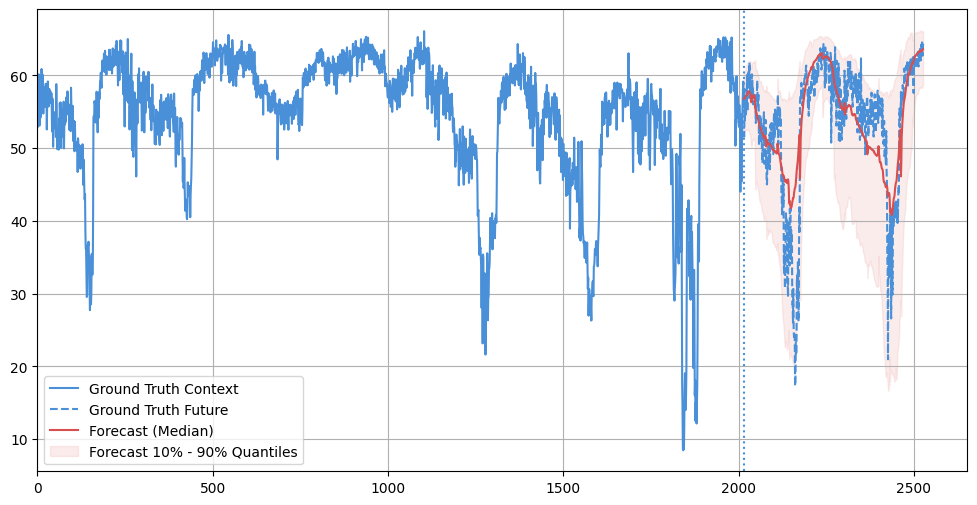
The long horizon forecast data example contains spatio-temporal speed information of the Seattle freeway system.

Make a forecast on the data, starting with a prediction length of 512

prediction_length = 512

ctx_l, future_l = np.split(pd.read_csv(f"{data_base_url}/loop_seattle_5T.csv").values.reshape(-1), [-prediction_length])
quantiles_l, mean_l = model.forecast(ctx_l, prediction_length=prediction_length)

print(f"Long series (spatio-temporal speed information of the Seattle freeway system): {prediction_length=}")
plot_forecast(context=ctx_l, ground_truth=future_l, forecasts=quantiles_l[0])

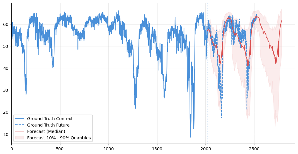
Extend the prediction length

# extend forecast length
prediction_length = 768

quantiles_l_768, mean_l_768 = model.forecast(ctx_l, prediction_length=prediction_length)
plot_forecast(context=ctx_l, ground_truth=future_l, forecasts=quantiles_l_768[0])

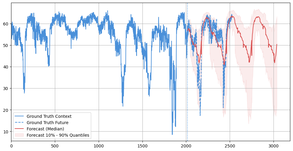
# extend forecast length
prediction_length = 1024

quantiles_l_1024, mean_l_1024 = model.forecast(ctx_l, prediction_length=prediction_length)
plot_forecast(context=ctx_l, ground_truth=future_l, forecasts=quantiles_l_1024[0])

6. Evaluate your Forecasts

Now that you have created some forecasts using TiRex its time to evaluate its prediction quality. This can be done using different metrics. A deeper discussion of common evaluation metrics is available in the Evaluation section.

def mape(x, ref):
  return np.mean(np.abs((np.array(ref) - np.array(x)) / np.array(ref))) * 100

def mae(x, ref):
  return np.mean(np.abs(np.array(ref) - np.array(x)))

def mse(x, ref):
  return np.mean((np.array(ref) - np.array(x)) ** 2)

def rmse(mse):
  return np.sqrt(mse)


# truncate forecast means to same length as future values
mean_s = mean_s[:, :future_s.shape[0]]
mean_l = mean_l[:, :future_l.shape[0]]

print(f"MAPE [%] short: {mape(mean_s, future_s):6.2f} long: {mape(mean_l, future_l):6.2f}")
print(f"MAE      short: {mae(mean_s, future_s):6.2f} long: {mae(mean_l, future_l):6.2f}")
print(f"MSE      short: {mse(mean_s, future_s):6.2f} long: {mse(mean_l, future_l):6.2f}")
print(f"RMSE     short: {rmse(mse(mean_s, future_s)):6.2f} long: {rmse(mse(mean_l, future_l)):6.2f}")

Example results (yours might look different) formated as table:

Metric	Short Horizon	Long Horizon
MAPE [%]	9.90	9.75
MAE	44.40	3.97
MSE	3787.37	34.29
RMSE	61.54	5.86